How Much Should You Order? A Stochastic Optimization Demo You Can Play With

Building an inventory-policy optimizer that reasons over thousands of possible futures, and shipping it as a live web app.

TL;DR I built a small web app that solves a textbook inventory problem in a slightly non-textbook way. Instead of choosing a reorder policy from a single demand forecast, it defines the problem over thousands of simulated futures and returns the policy with the best expected outcome across all of them. It runs on three real point-of-sale datasets (Walmart, UCI Online Retail), shows the full cost-vs-reliability tradeoff, and explains its recommendation in plain English. Try it live at inventory.christopherrobertwhite.com, or read the code on GitHub.

The one-forecast problem

Say you run inventory for one SKU and get handed a demand forecast: "about 12 units a day." Fine. Five-day lead time means you'll sell about 60 units during the wait, so you reorder at 60.

Then Tuesday happens and you sell 34.

That's the problem with planning off a point forecast: it's right on average, and average is the wrong thing to plan against. What matters is the shape of the distribution. A quiet SKU with low variance needs almost no safety buffer. A bursty one with occasional 4,000-unit spikes needs a much bigger buffer, or an honest acknowledgment that you'll stock out sometimes because covering every spike would eat your entire margin.

Operations research solved this a long time ago: optimize against a distribution of possible futures instead of a single point estimate, and pick the policy that performs best across all of them, weighted by how likely each future is. That's what the demo does.

What I built

A three-page web app that lets you:

1. Pick one of three real POS scenarios (a steady Walmart pantry item, an intermittent Walmart hobbies item, and a heavy-tailed UK gift-shop item from UCI Online Retail II).
2. Configure lead-time uncertainty and pick a reliability target.
3. Click Optimize. The backend scores a grid of about 240 candidate reorder policies against 1,000 Monte Carlo simulations of a 180-day future, and returns the cheapest policy that meets your reliability target.
4. Inspect the result: the recommended policy in plain English, the full cost-vs-reliability Pareto frontier, a fan chart of simulated inventory paths, and a side-by-side comparison against textbook rules.

Try it here: inventory.christopherrobertwhite.com

The stack is FastAPI plus NumPy on the backend, React plus Vite plus TypeScript on the frontend, Docker to Google Cloud Run for hosting, and Cloudflare for DNS. The full method write-up (mermaid diagrams, math, an honest comparison to solver-based alternatives) is in FORMULATION.md on the repo.

The core idea in one paragraph

You have a reorder policy $\pi$ (for example: "when inventory drops to 60 units, order 100 more"). You have random future daily demand $D_t$ and random lead times $L_i$. Under any given policy, your total cost $C(\pi)$ for a 180-day horizon is a random variable, driven by holding cost, ordering cost, and stockout penalties. Instead of optimizing against a single deterministic future, you optimize the expected cost across many random ones, subject to a reliability constraint you choose:

$$\begin{aligned} \text{minimize} \quad & \mathbb{E}[C(\pi)] \\ \text{subject to} \quad & \Pr(\text{stockout on any day} \mid \pi) \le 1 - \alpha \end{aligned}$$

α is your reliability target: 95%, 99%, whatever your business tolerates. The expectation is approximated by the sample mean over N=1,000 simulated futures, a standard technique in stochastic programming called Sample Average Approximation (SAA). Everything else in the app is engineering around that one formulation.

Why not just use a solver?

Purists might raise an eyebrow at "grid search plus Monte Carlo" instead of a proper mixed-integer program handed to Gurobi. Here's why I didn't.

The policy space is small to begin with. A reorder policy is two integers, r and Q (or r and S for order-up-to policies), each with maybe a couple hundred plausible values. That's a few thousand candidates before deduping, and my vectorized NumPy simulator scores the whole grid in one to two seconds. Grid search lands within one unit of the true optimum, no big-M constraints, warm-start heuristics, or license fees required.

The dynamics are also non-convex. Inventory is a piecewise function of past demand and past orders, and threshold-triggered ordering is a discrete event. You can encode that in an MIP, but the model gets ugly fast, and solve time balloons for reasons that have more to do with modeling than math.

And the demand distribution is empirical: real POS data is bursty, has zero-days, and doesn't fit a clean parametric family. A solver-based formulation would still need to reduce that empirical distribution to a finite set of scenarios, which is SAA anyway. Might as well skip the middleman and simulate directly.

What "reliability" actually costs

The single most useful visualization in the app is the cost-vs-reliability frontier. Every candidate policy is a dot on a scatter plot. The x-axis is expected monthly cost. The y-axis is the probability a random day ends without a stockout.

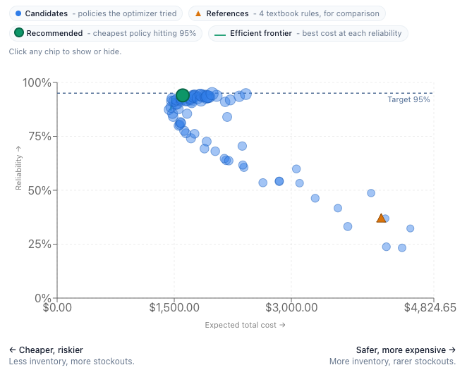
The upper-left edge of that cloud is the Pareto frontier: the set of policies that aren't dominated by anything else. If a policy is on the frontier, no other policy in the grid gives you more reliability at the same cost, or the same reliability at lower cost. Everything below the frontier is strictly worse and can be ignored.

Once you can see the frontier, one of the app's headline lessons appears immediately: the last 5% of reliability costs a lot. Going from 90% to 95% might cost you 20% more inventory. Going from 95% to 99% might double the inventory bill. On the heavy-tailed UK scenario, 99% isn't reachable at any cost, because the demand distribution has a fat enough tail that no finite buffer covers every spike.

This isn't a novel observation in OR, but it's new to almost every non-specialist I've shown the app to. Getting people to feel that reliability has a real dollar cost attached to it, not just a customer-service platitude, was the actual design goal here.

Three real scenarios, three lessons

I resisted the temptation to ship ten scenarios. Three is enough to teach the story, and each one is deliberately chosen to break a different intuition:

1. walmart_pantry_m5: a Walmart Los Angeles pantry item, about 12 units per day, roughly 5% zero-days. The clean baseline. The optimizer's recommendation matches what a well-tuned Newsvendor-style rule would tell you, and the frontier has a nice smooth shape. Useful as an anchor.

2. walmart_hobbies_sparse_m5: another Walmart LA item, but hobbies, and very slow-moving. About 85% zero-days, roughly 0.2 units per day on average. Here the intuition-breaker is that cycle service level (the probability of no-stockout on a given day) and fill rate (the fraction of demanded units served) diverge sharply. A policy can hit 95% reliability at very low cost simply because most days have zero demand, but that number is misleading. Fill rate tells a truer story for intermittent SKUs.

3. retail_online_uk: a heavy-tailed UK gift-shop item from UCI Online Retail II. The median day sells 88 of them; the biggest day sells over 4,000. The closest the optimizer gets here is about 93.5% cycle service level (a 6.5% stockout probability), short of the 95% target. Fill rate on that same policy is 99.7%, a reminder of how differently the two metrics can read even on the scenario built to break cycle service level. The app surfaces this explicitly and suggests fill rate as the better metric here.

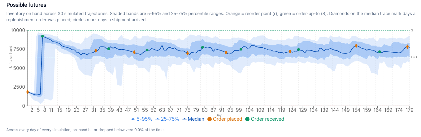
Notice the caption on that chart: zero stockouts across all 30 sampled paths, even though the real stockout probability is 6.5%. That's not a contradiction, it's the whole reason to run a thousand simulations instead of eyeballing a handful. A small sample can look perfectly safe right up until it isn't.

I think a portfolio app is more useful when it can articulate the limits of its own method. This one tries to.

Design decisions

• Real data over synthetic curves. Every demand history in the app is real POS data; only the cost assumptions are illustrative. Portfolio demos that generate their own bell curves always felt a little dishonest to me, real data has zero-days, outliers, and weekly seasonality that a model actually has to handle.

• Progressive disclosure. I built the full parameter set first, then hid two-thirds of it behind an "Advanced" panel once I saw how much better the default view read for a non-specialist. The four inputs that actually matter (scenario, lead time, costs, reliability target) are what you see first.

• An explicit optimize button. Early versions re-optimized on every parameter change. It felt responsive but was disorienting, nobody could tell which knob caused which effect. Now it runs once, on click, with a phase-based progress bar.

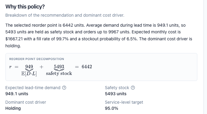
• An explainability panel. Every recommendation breaks down into plain English: expected demand during the lead time, how much of the reorder point is safety stock, which cost component dominates, and how it compares to four textbook reference rules.

• The notebook, too. Same optimizer, same domain layer, exposed end-to-end in a Jupyter notebook for anyone who'd rather read Python than click through a UI. Every parameter at the top, every intermediate visualized, no server required.

What I'd change next

A few honest limitations, if this were headed to production instead of a portfolio. The policy grid is discrete; a continuous version would move to something like SPSA, not hard, but not necessary at this scale, until the SKU catalog gets much larger. It only handles one SKU at a time, and real inventory decisions are joint: shared warehouse capacity, joint reorder cycles, substitution effects between SKUs. That's a genuinely different class of problem (multi-echelon, capacitated) and the interesting next step. Costs are also illustrative: in the real world, unit cost is a negotiation, holding cost gets mis-attributed constantly, and stockout penalty is a business-strategy conversation, not a number. The app makes all three editable, which is the honest thing to do, but if I were consulting on a real deployment, the first workshop would be "what is your stockout actually worth." And the empirical bootstrap assumes stationarity, so there's no demand drift modeled: a production version would need to handle seasonality changes, promotions, and stockouts suppressing the training data itself.

Try it, or read the code

• Live demo: inventory.christopherrobertwhite.com
• GitHub repo: chrisrwhite/stochastic-inventory-explorer
• Math and methodology: FORMULATION.md has the full model, mermaid diagrams of the pipeline and simulation loop, and an honest comparison to solver-based alternatives.
• Notebook walkthrough: the same pipeline as a Jupyter notebook, every parameter at the top, matplotlib plots inline.
• Data provenance: DATA_LICENSES.md

If you try it and a recommendation feels wrong, or you build something on top of it, let me know. I'd genuinely like to hear about it.